10. Differential pseudotime and receptor ranking

Language: Python · Input: delta embeddings from step 9 · Output: receptor_scores.csv, receptor score heatmap and barplots, per-receptor vector fields

In this step, we will turn the simulated knockouts into a ranking of the receptors. For each receptor, differential_pseudotime_analysis reads its delta embedding, smooths the displacement vectors onto a user defined grid, and projects every cell’s displacement onto the local pseudotime gradient. The result is how far along the trajectory each cell moves when the receptor is knocked out, which the function scores per receptor with Cohen’s d and a Wilcoxon signed-rank p-value — once over all MSCs and once per subcluster.

A positive score means the cells shift towards the OLCs, a negative score means they shift back towards the Adipo-CAR state.

import scanpy as sc
from intratalkerpy.perturbation import mt, pl

COND = "KO"

data      = sc.read_h5ad(PERT / f"MSCs_diffmap_{COND}_subset.h5ad")
sim_path  = PERT / f"MSCs_{COND}" / "simulation"
save_path = PERT / f"MSCs_{COND}" / "results"

data = mt.differential_pseudotime_analysis(
    data,
    folder_path = sim_path,
    save_path   = save_path,
    red_namem   = "X_diffmap",
    cell_anno   = "sub_annotation",
    pseudo_name = "dpt_pseudotime",
    grid_size   = 25,
    offset_frac = 0.005,
    n_neigh     = 10,
)

The returned object carries the results of all receptors:

Field	Contents
obs["pseudotime_{receptor}"]	perturbed pseudotime, one column per receptor
uns["receptor_scores"]	Cohen’s d and Wilcoxon p-values, over all cells and per subcluster
uns["vector_fields"]	the smoothed displacement field of each receptor, plotted below

The results are written to disk as well

Besides returning the object, the function writes it into save_path as differential_pseudotime.h5ad, so we can come back to the scores and the vector fields later without running the analysis again. output_name gives the file another name, which is worth setting when the results of both conditions end up in the same folder.

Receptor scoring heatmap

The heatmap shows Cohen’s d for every receptor across the MSC subclusters, so we can see whether a receptor moves the whole compartment or only one state. With save_csv=True the underlying table is written as receptor_scores.csv, which the barplot below reads.

pl.plot_score_heatmap(
    data.uns["receptor_scores"], str(save_path),
    max_score_limit     = 2.0,
    cmap                = "coolwarm",
    significance_method = "pval",
    cluster_rows        = True,
    cluster_cols        = False,
    save_csv            = True,          # -> receptor_scores.csv
)

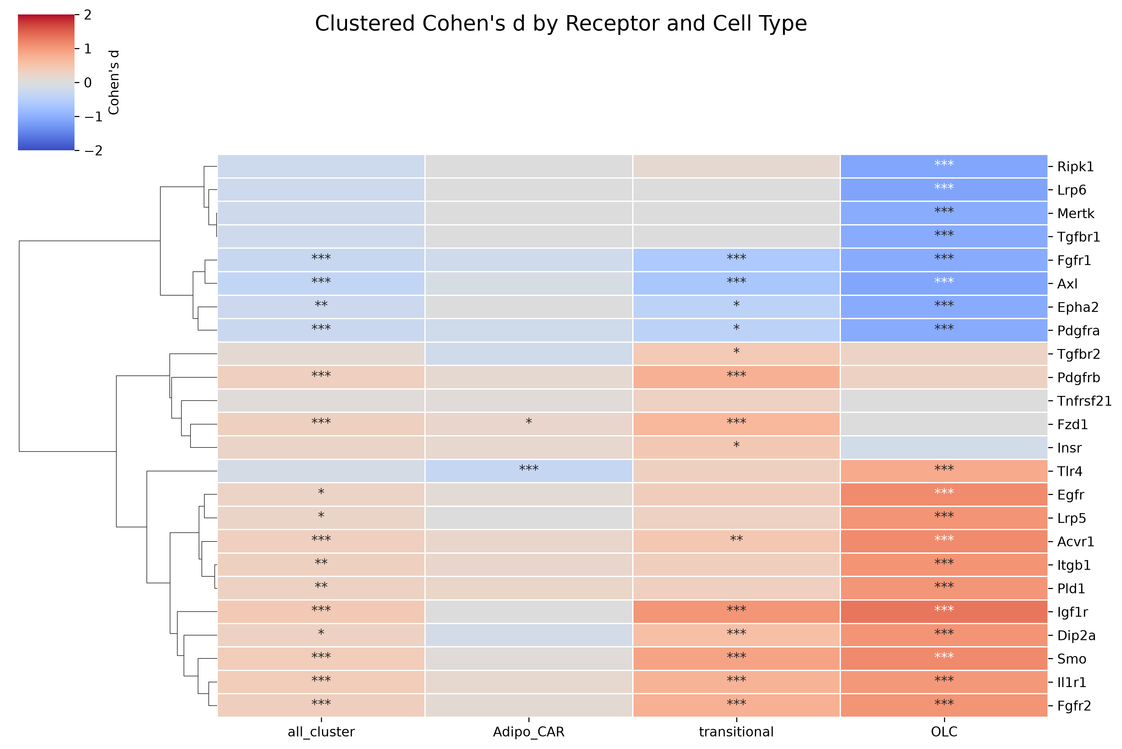
Cohen’s d of the 24 simulated knockouts in the KO cells, over all MSCs (all_cluster) and per subcluster; stars mark the Wilcoxon p-value. The row clustering splits the receptors into a block that pushes the cells backwards along the trajectory (blue in the OLC column: Ripk1, Lrp6, Mertk, Tgfbr1, Fgfr1, Axl, Epha2, Pdgfra) and a block that pushes them forwards (Il1r1, Igf1r, Smo, Fgfr2, Acvr1, Egfr, …).

Most of the signal sits in the transitional and OLC columns; the Adipo-CAR cells sit at the root of the trajectory and barely move under any knockout except Tlr4. Keep the cell numbers in mind when reading the per-subcluster columns — in the KO subset the OLC state holds 26 cells, so a large Cohen’s d there rests on few cells.

Top receptors by perturbation score

pl.plot_score_barplots(
    data.uns["receptor_scores"], str(save_path),
    cohens_d_threshold = 0.0,
    top_n              = 10,
    fig_width          = 15,
    fig_height         = 6,
)

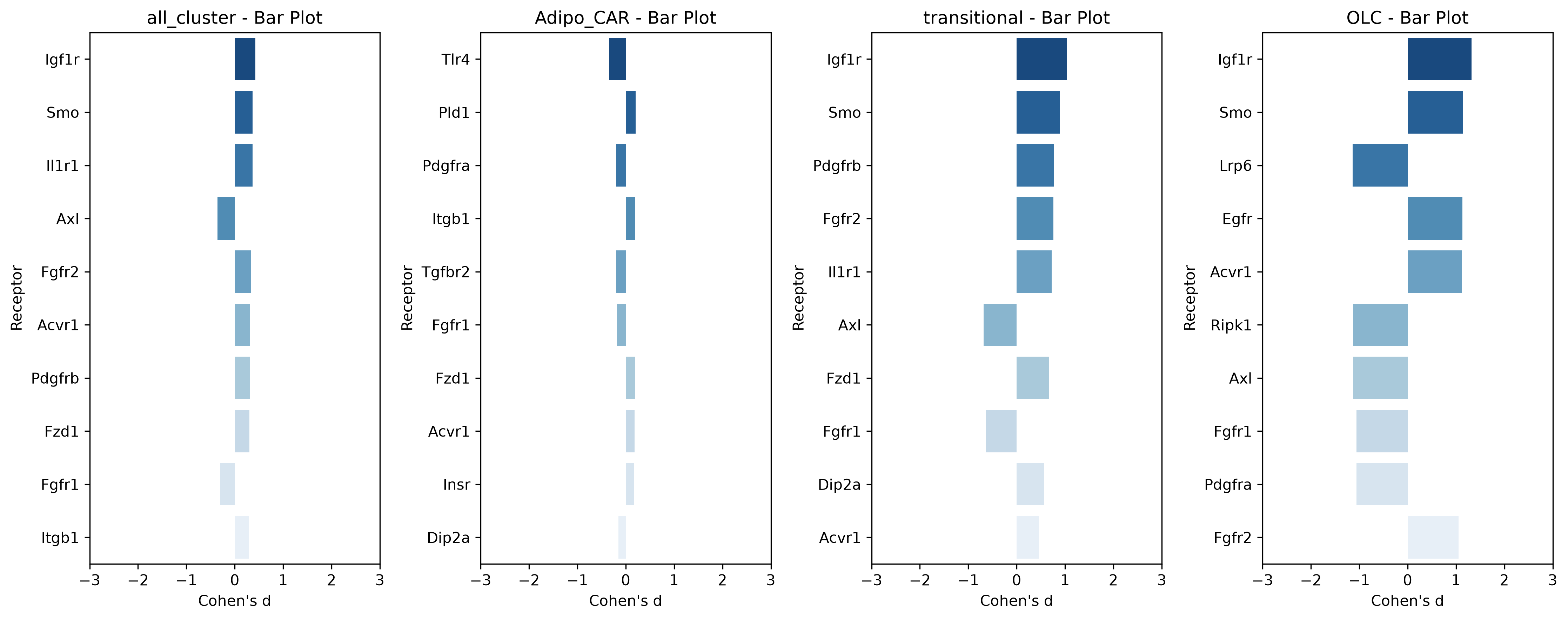
The ten strongest effects per column of the heatmap, ranked by |Cohen’s d|. Igf1r and Smo lead in every column they appear in; Il1r1 is third over all MSCs and fifth in the transitional state.

cohens_d_threshold drops the weak effects before ranking — at 0.0 every simulated receptor is a candidate, raising it to 0.5 keeps only the receptors that move their subcluster by half a standard deviation or more.

Vector fields of the simulated knockouts

The scores compress each knockout into a single number. The vector fields show where on the trajectory the cells actually moved, which is what tells apart a receptor that pushes the whole compartment from one that only acts locally.

differential_pseudotime_analysis already computed them — uns["vector_fields"] holds one entry per receptor:

Key	Contents
grid_points	the 25 × 25 grid laid over the diffusion map, shape (625, 2)
vectors	the Gaussian-smoothed displacement at each grid point; NaN where no cells lie underneath the grid point or the displacement is negligible
distances	the length of each displacement vector, used to shade the streamlines
original_vectors	the unsmoothed per-cell displacements read from the delta CSV
mask	which grid points have cells underneath them

Two functions turn this into a figure: plot_differential_pseudotime colours every cell by how far it moved along the trajectory, and vector_field_wrapper draws the smoothed displacements as streamlines over the diffusion map. For a single receptor, we can plot the vector field like this:

RECEPTOR = "Il1r1"
v = vectors[RECEPTOR]

fig, ax = plt.subplots(figsize=(7.5, 6))
ax = pl.vector_field_wrapper(
    data,
    v["grid_points"],
    v["vectors"],
    v["distances"],
    "X_diffmap", "sub_annotation", RECEPTOR,
    color_dictionary, ax=ax,
    grid_dist      = 25,
    stream_density = 2,
)

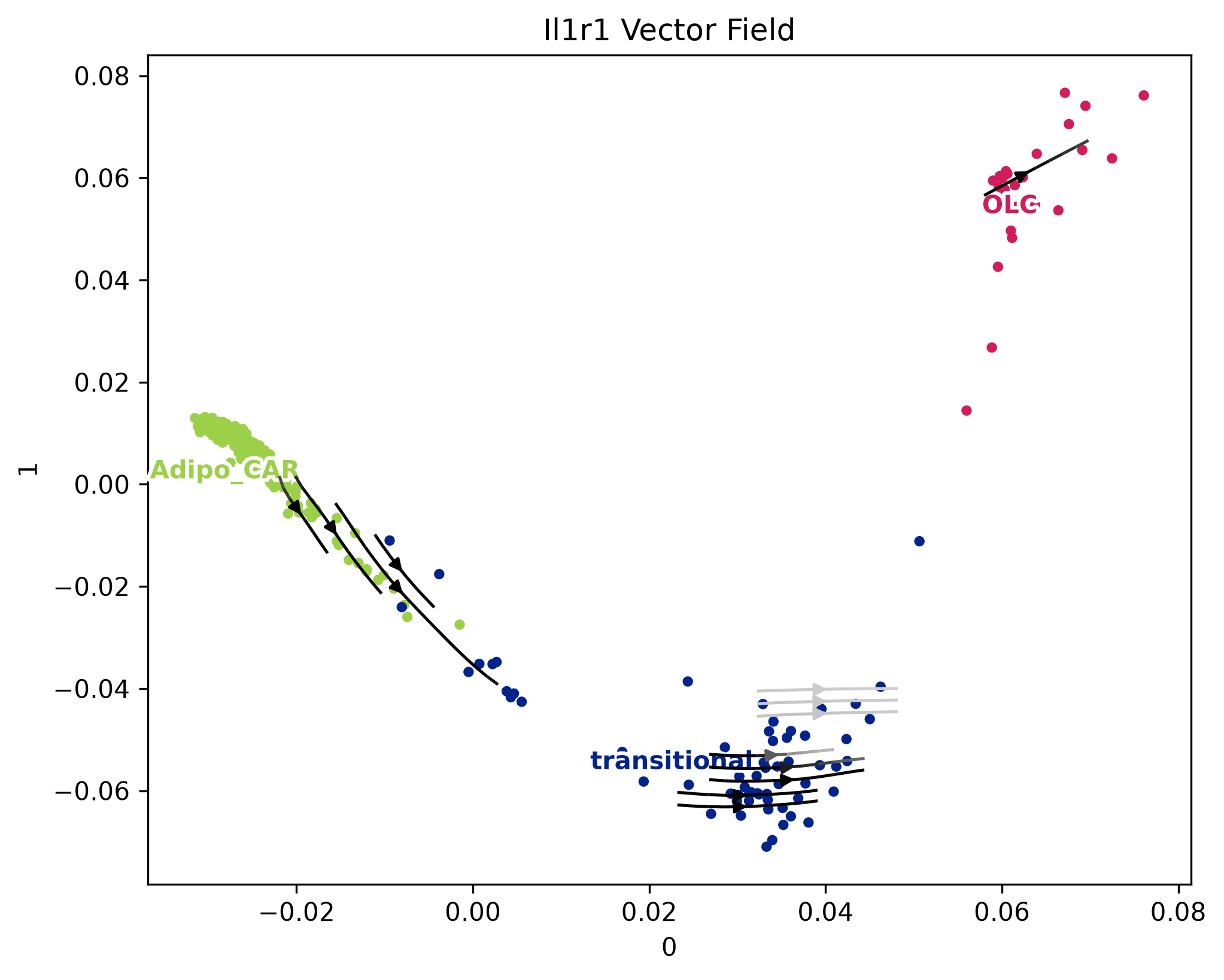
The Il1r1 knockout in the Il1rn KO cells. The streamlines run along the trajectory in the direction of increasing pseudotime — from the Adipo-CAR cells, through the transitional state, and onwards to the OLCs.

Removing Il1r1 in the KO cells shifts the compartment forwards along the trajectory, and the shift is carried by the cells that have already left the Adipo-CAR state: it is significant in the transitional state and in the OLCs, while the Adipo-CAR cells hardly shift. Running the same block on the WT results gives the panel to compare it against.

grid_dist has to match grid_size

vector_field_wrapper reshapes the flat grid to (grid_dist, grid_dist, 2) before handing it to streamplot, so it has to be the grid_size that differential_pseudotime_analysis ran with — 25 here. Any other value fails in the reshape.

Expected result

Il1r1 comes out among the strongest receptors in the KO cells, and it moves the MSCs along the Adipo-CAR → osteolineage axis — the in silico counterpart of the differentiation shift the Il1rn knockout causes in the data.

Repeating step 9 and this step on the WT subset gives the second half of the comparison the case study is built on: the Il1r1 effect is markedly larger in KO than in WT cells, as expected for a receptor that is activated once its antagonist Il1rn is gone. If Il1r1 does not separate between the conditions, check that the Il1rn → Il1r1_Il1rap interaction really made it into the LR table (step 2).

Next: Session info