4. IntraTalker + CrossTalkeR2

Language: R · Input: integrated .h5ad, mouse_dorothea_AB.csv, decoupler_dorotheaAB_results_ulm.csv, KO_lr_ready.csv, WT_lr_ready.csv · Output: result_TF_object.RDS, LR_data_final.Rds, edges_directed_KO_WT_filtered.csv

In this step, you will combine the ligand–receptor interactions generated in Python with transcription factor activities to reconstruct intracellular signalling networks. These networks are then integrated into CrossTalkeR2 to build condition-specific cell–cell communication networks and differential network statistics.

The analysis uses IntraTalker and CrossTalkeR v2.

Load the integrated dataset

The remaining analysis is performed in R. Start by loading the integrated .h5ad file as a Seurat object using anndataR.

library(anndataR)
library(Seurat)

BASE    <- "/path/to/Il1rn_KO"
DATA    <- file.path(BASE, "data")
LR_OUT  <- file.path(BASE, "lr")
TF_OUT  <- file.path(BASE, "tf")
CTR_OUT <- file.path(BASE, "crosstalker")

data.object <- read_h5ad(
  file.path(DATA, "bone_marrow_Il1rn_KOvsWT_harmony_integrated.h5ad"),
  as = "Seurat"
)

Identify differentially active transcription factors

IntraTalker_analysis() reads the transcription factor activities generated by decoupleR in the previous step. It does not recompute them. Instead, it tests for differential TF activity between KO and WT within each cell type and constructs intracellular receptor → transcription factor → target gene networks.

The parameters below reproduce the analysis from the publication, using cluster-wise t-tests with a significance threshold of p < 0.01 and a minimum logFC > 0.4.

library(IntraTalker)
library(CrossTalkeR)

parameters <- list(
  out_path        = TF_OUT,
  reg             = file.path(TF_OUT, "mouse_dorothea_AB.csv"),
  organism        = "mouse",
  celltype        = "cluster_names",
  condition       = "Condition",
  comparison_list = list(c("KO", "WT")),
  logfc           = 0.4,
  pval            = 0.01,
  test_type       = "t",
  Seurat          = FALSE
)

results <- IntraTalker_analysis(
  seuratobject   = data.object,
  tf_activities  = file.path(TF_OUT, "decoupler_dorotheaAB_results_ulm.csv"),
  arguments_list = parameters
)

The resulting object is written to

TF_OUT/TF_results/result_TF_object.RDS

and contains the intracellular signalling networks for both conditions. These networks are the input of the receptome step, which runs in Python — step 7 starts with the few lines that export them as CSV.

Combine intracellular and intercellular signalling

Next, merge the intracellular signalling networks with the ligand–receptor interactions generated by LIANA+. Receptor complexes (for example Il1r1_Il1rap) are preserved throughout the analysis.

LR_KO <- read.csv(file.path(LR_OUT, "KO_lr_ready_custom.csv"), row.names = 1)
LR_WT <- read.csv(file.path(LR_OUT, "WT_lr_ready_custom.csv"), row.names = 1)

KO_combined <- combine_LR_and_TF(
  results@CTR_input_condition$KO,
  unique(LR_KO),
  CTR_OUT,
  "KO",
  consider_complexes = TRUE
)

WT_combined <- combine_LR_and_TF(
  results@CTR_input_condition$WT,
  unique(LR_WT),
  CTR_OUT,
  "WT",
  consider_complexes = TRUE
)

This step also creates the files

• CrossTalkeR_input_KO.csv

• CrossTalkeR_input_WT.csv

which serve as the input for CrossTalkeR2.

Generate the CrossTalkeR2 report

Finally, generate the integrated communication networks and the accompanying HTML report.

paths <- list(
  KO = file.path(CTR_OUT, "CrossTalkeR_input_KO.csv"),
  WT = file.path(CTR_OUT, "CrossTalkeR_input_WT.csv")
)

CTR_data <- generate_report(
  paths,
  out_path     = CTR_OUT,
  threshold    = 0,
  out_file     = "Il1rn_KO_vs_WT.html",
  output_fmt   = "html_document",
  org          = "mmu",
  comparison   = list(c("KO", "WT")),
  p_val        = 0.05,
  filtered_net = TRUE
)

This produces both the interactive HTML report and the final CrossTalkeR object (LR_data_final.Rds), which is used throughout the remaining tutorial.

Export the edge table for the cell–cell network community detection

The community detection and layout happens in Python (step 6); R only exports the differential cell–cell network as a flat edge list.

# the Fisher-filtered network -- this is the one used in the publication
write.csv(igraph::as_data_frame(CTR_data@graphs[["KO_x_WT_filtered"]], what = "edges"),
          file.path(CCI_LAYOUT, "edges_directed_KO_WT_filtered.csv"), row.names = FALSE)

The result is a CSV with from, to, weight — one row per sender→receiver cell pair, weight = differential LR score (KO − WT).

The original CrossTalkeR CCI plot

With the plot_cci function we can draw the cell–cell network directly in R, with Pagerank-scaled node sizes and a circular layout.

plot_cci(
    CTR_data@graphs[["KO_x_WT_filtered"]],
    paste0(""),
    emax                = NULL,
    leg                 = FALSE,
    low                 = 0,
    high                = 0 / 100,
    ignore_alpha        = FALSE,
    log                 = TRUE,
    efactor             = 5,
    vfactor             = 12,
    vnames              = TRUE,
    pg                  = CTR_data@rankings[["KO_x_WT_filtered"]]$Pagerank[
                            V(CTR_data@graphs[["KO_x_WT_filtered"]])$name],
    vnamescol           = NULL,
    colors              = CTR_data@colors[V(CTR_data@graphs[["KO_x_WT_filtered"]])$name],
    coords              = CTR_data@coords[V(CTR_data@graphs[["KO_x_WT_filtered"]])$name, ],
    col_pallet          = c("#3B4CC0", "#F2F2F2", "#DD0029"),
    standard_node_size  = 10,
    pg_node_size_low    = 10,
    pg_node_size_high   = 40,
    arrow_size          = 0.7,
    arrow_width         = 1.5,
    node_label_position = 1.2,
    node_label_size     = 1
  )

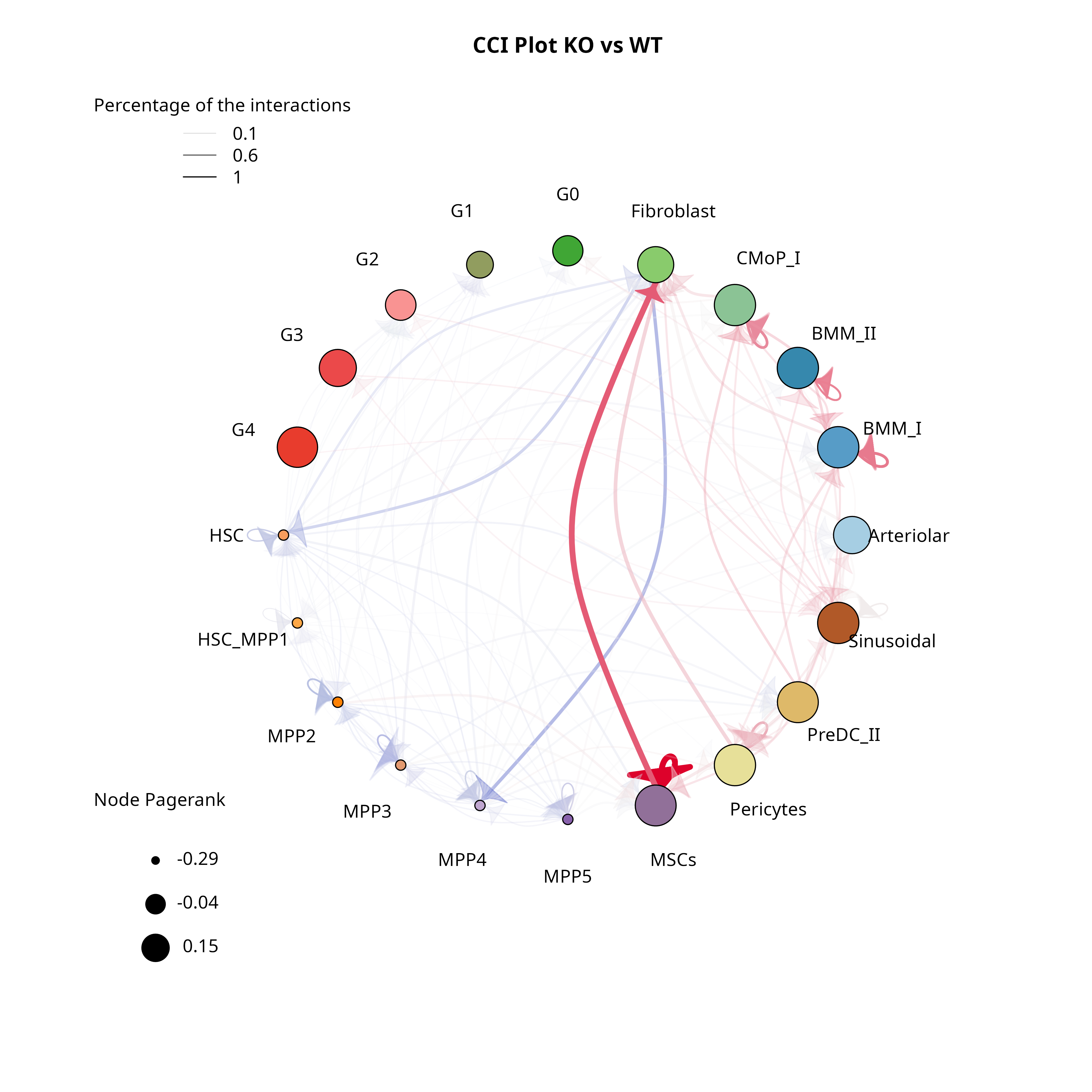
CrossTalkeR CCI plot KO vs WT conditions.

Verify the output

At this point, your output directory should contain

• TF_results/result_TF_object.RDS

• intracellular_network_{KO,WT}.csv (exported in step 7)

• CrossTalkeR_input_KO.csv

• CrossTalkeR_input_WT.csv

• LR_data_final.Rds

• Il1rn_KO_vs_WT.html

In the next step, we will plot the inter- and intracellular interactions of interest.

Next: Sankey Plots