1. Introduction and Setup

The workflow spans two languages. LR inference, TF activity, community detection, receptome construction, trajectory analysis and all perturbation simulations run in Python; the IntraTalker/CrossTalkeR integration and the Sankey figures run in R. The two sides never share objects in memory — they only exchange CSV / RDS files on disk. Every switch between them is marked with a HANDOFF section that lists exactly which files cross the boundary, so you can run either half independently as long as the handoff files exist.

First, all necessary Python and R libraries need to be installed.

Python environment

python -m venv .venv && source .venv/bin/activate
pip install scanpy scikit-learn seaborn adjustText statsmodels \
            networkx python-igraph leidenalg \
            pycrosstalker liana decoupler
pip install git+https://github.com/CostaLab/IntraTalkerpy.git

R environment

install.packages(c("Seurat", "igraph", "ggraph", "ggplot2", "dplyr", "tidyr",
                   "ggalluvial", "colorBlindness", "colorspace", "oce", "scales", "remotes"))
remotes::install_github("CostaLab/CrossTalkeR")   # v2.0.0
remotes::install_github("CostaLab/IntraTalker")   # v0.1.0

Paths

Every Python page assumes this block. Set BASE once.

from pathlib import Path

BASE       = Path("/path/to/Il1rn_KO_project")
DATA       = BASE / "data"          # input h5ad + regulon
LR_OUT     = BASE / "lr"
TF_OUT     = BASE / "tf"
CTR_OUT    = BASE / "crosstalker"
PERT       = BASE / "perturbation"

for p in (LR_OUT, PERT, PLOTS):
    p.mkdir(parents=True, exist_ok=True)

The R pages use the same layout via BASE <- "/path/to/Il1rn_KO":

from pathlib import Path

BASE       <- "/path/to/Il1rn_KO_project"
DATA       <- paste0(BASE, "/data")          # input h5ad + regulon
LR_OUT     <- paste0(BASE, "/lr/")            # steps 1-2   (Python -> R)
TF_OUT     <- paste0(BASE, "/tf/")            # step 3      (written by R)
CTR_OUT    <- paste0(BASE, "/crosstalker")   # step 3      (written by R)
PERT       <- paste0(BASE, "/perturbation")

Input data

Two objects are available on Zenodo (https://doi.org/10.5281/zenodo.20813791):

File	Used by
bone_marrow_Il1rn_KOvsWT_harmony_integrated.h5ad	steps 2–3, and the UMAP below
bone_marrow_Il1rn_KOvsWT_MSCs_trajectory.h5ad	steps 8–10, the perturbation analysis

The first is the Harmony-integrated data set of all 20 cell types. Its relevant annotation is stored in the obs columns cluster_names (20 cell types) and Condition (KO / WT).

The second is its MSC compartment with the sub-populations, the diffusion map and the pseudotime of the publication — the trajectory the receptor knockouts are projected onto. We provide it ready to use so that the perturbation half of the tutorial can be run on its own; see step 8.

We can visualise the data with a UMAP:

import scanpy as sc
import matplotlib.pyplot as plt

adata = sc.read("bone_marrow_Il1rn_KOvsWT_harmony_integrated.h5ad")
adata.obs["cluster_names"] = adata.obs["cluster_names"].astype("category")

group_map = {   # colourblind-safe, grouped by lineage
    "G0": "#08306b", "G1": "#08519c", "G2": "#2171b5", "G3": "#4292c6", "G4": "#6baed6",
    "MPP2": "#e69f00", "MPP3": "#f0a202", "MPP4": "#f6c141", "MPP5": "#f8d97b",
    "BMM_I": "#009e73", "BMM_II": "#03f0b1",
    "MSCs": "#cc79a7", "Fibroblast": "#d52e00", "CMoP_I": "#e69f00",
    "PreDC_II": "#7b3294", "Arteriolar": "#f0e442", "Pericytes": "#a6761d",
    "HSC": "#66a61e", "HSC_MPP1": "#4c7b16", "Sinusoidal": "#56e4e9",
}
palette = [group_map[g] for g in adata.obs["cluster_names"].cat.categories]

sc.pl.embedding(adata, basis="umap", color="cluster_names",
                palette=palette, ax=ax, show=True, frameon=True, size=8)

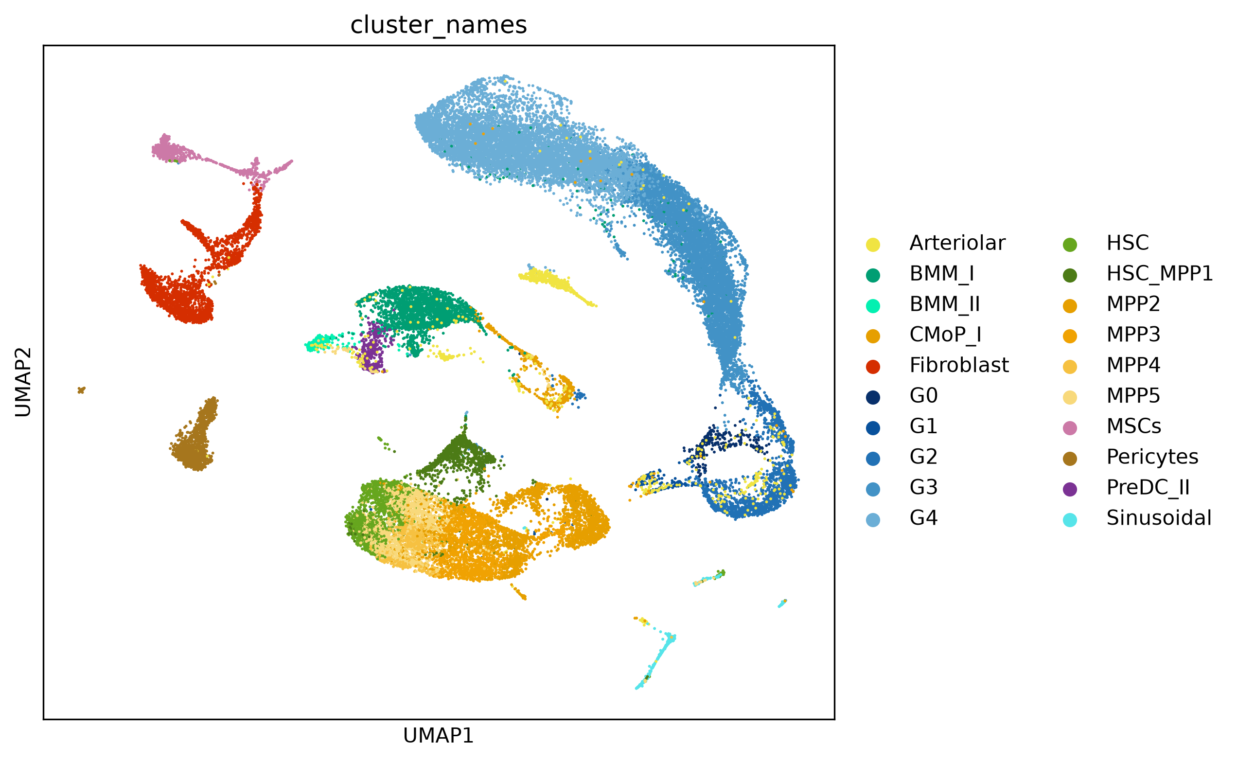
UMAP of the integrated Il1rn KO data set.

In the next step, we perform ligand–receptor interaction predictions: Next: Ligand–receptor inference