8. The MSC trajectory object

Language: Python · Input: bone_marrow_Il1rn_KOvsWT_MSCs_trajectory.h5ad · Output: MSCs_diffmap_{WT,KO}_subset.h5ad

The receptor knockouts of the next two steps are projected into a two-dimensional embedding of the MSC compartment, and every score is read off a pseudotime defined on it. The embedding is therefore not an illustration but part of the analysis.

For convenience we prepared that object for you: bone_marrow_Il1rn_KOvsWT_MSCs_trajectory.h5ad on Zenodo is the MSC compartment of the integrated data set, with the sub-populations of the publication, a diffusion map and a diffusion pseudotime — both computed with scanpy (sc.tl.diffmap, sc.tl.dpt).

In this step we load that object and take a look at the data. Working on your own data, you can bring any 2-D trajectory and any pseudotime instead — see 8.1 below.

8.1 Load the trajectory

import scanpy as sc

msc = sc.read_h5ad(DATA / "bone_marrow_Il1rn_KOvsWT_MSCs_trajectory.h5ad")
msc

AnnData object with n_obs × n_vars = 828 × 27998
    obs: 'nCount_RNA', 'nFeature_RNA', 'SampleName', 'SampleGroup', 'Condition',
         'cell_group', 'cluster_names', 'cluster_condition', 'leiden_msc',
         'sub_annotation', 'dpt_pseudotime'
    var: 'highly_variable'
    uns: 'cell_group_colors', 'cluster_names_colors', 'diffmap_evals', 'iroot',
         'iroot_cell', 'leiden_msc', 'leiden_msc_colors', 'neighbors', 'pca',
         'provenance', 'sub_annotation_colors'
    obsm: 'X_diffmap', 'X_pca', 'harmony', 'pca', 'umap', 'umap.integrated_harmony'
    varm: 'PCs'
    layers: 'counts'
    obsp: 'connectivities', 'distances', 'nn', 'snn'

The fields the perturbation steps depend on:

Field	Contents
obsm["X_diffmap"]	DC1 and DC2, the embedding the knockouts are projected into
obs["sub_annotation"]	the three MSC states, in trajectory order
obs["dpt_pseudotime"]	diffusion pseudotime, scaled 0–1, increasing with DC1
obs["Condition"]	WT (516 cells) / KO (312 cells)
uns["sub_annotation_colors"]	the palette of the figures — scanpy picks it up on its own
uns["provenance"]	how the object was built, in prose
X / layers["counts"]	log-normalised expression / raw UMI counts

obsm["pca"], harmony, umap and umap.integrated_harmony are inherited from the integrated object of step 1 and were computed on all of its cells; X_pca and X_diffmap are the MSC-level embeddings the trajectory is built on.

Bring your own trajectory

Nothing in the perturbation steps is specific to a diffusion map. The functions take the embedding, the pseudotime and the cell annotation by name — project_perturbation_in_embedding(..., reduction_name=...) in step 9 and differential_pseudotime_analysis(..., red_namem=..., pseudo_name=..., cell_anno=...) in step 10 — so a UMAP, a PHATE or a force-directed embedding works just as well, with a pseudotime from the method of your choice.

Two requirements: the embedding in obsm has to be two-dimensional (the displacement vectors and the streamlines live in the plane), and the pseudotime has to be a numeric column in obs. The sub-population labels are only used to group the scores, so any categorical obs column will do.

8.2 The trajectory

The three sub-populations lie along one continuous arc in the diffusion map rather than in separate islands — the differentiation gradient the knockouts are scored against.

sc.pl.embedding(
    msc,
    basis="diffmap",
    color="sub_annotation",
    components="1,2",      # X_diffmap holds exactly DC1 and DC2
    size=55,
)

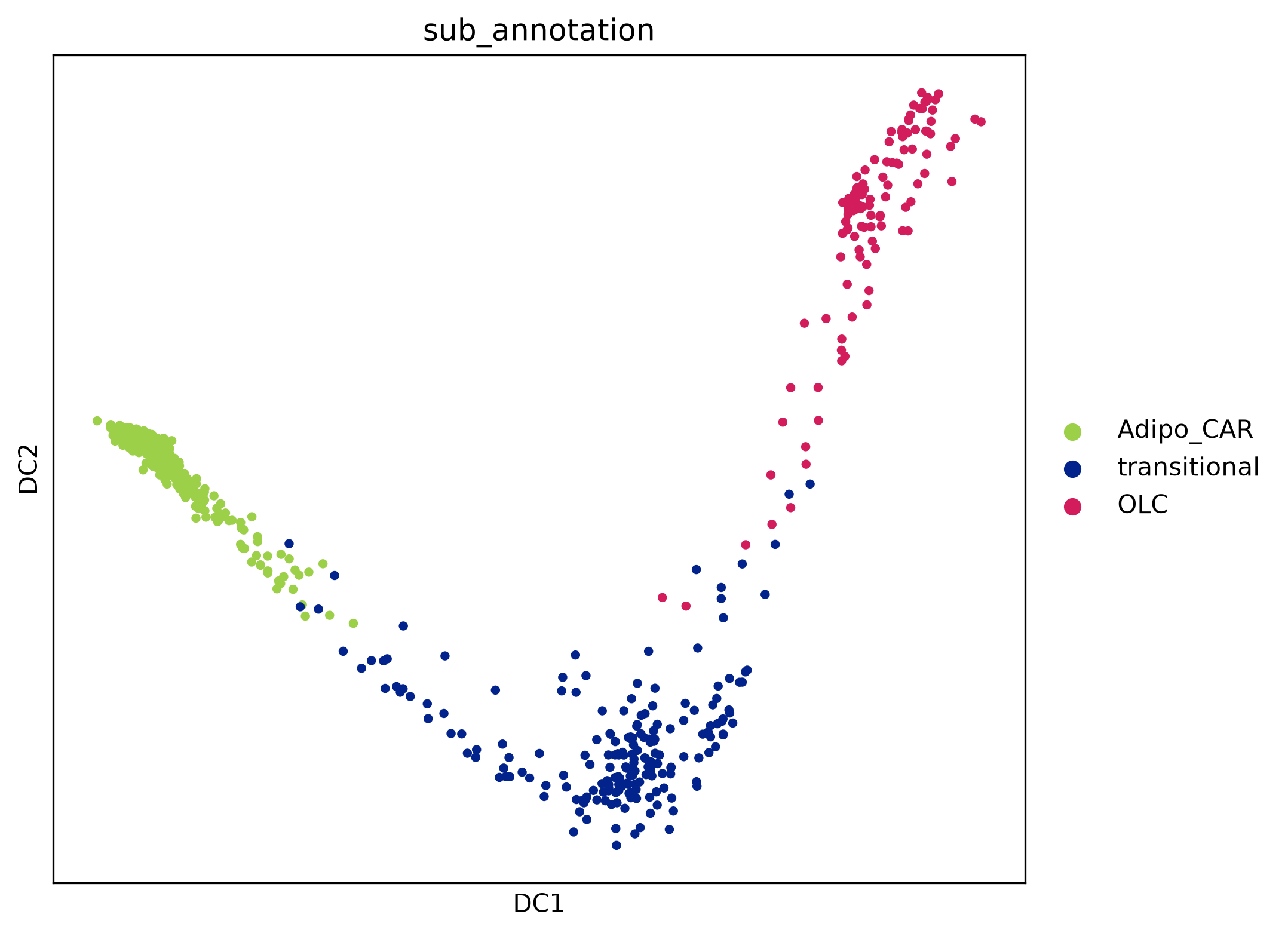
The MSC compartment in DC1/DC2: Adipo-CAR (518 cells), transitional (196) and OLC (114).

Colouring the same embedding by pseudotime reveals that the Adipo-CAR cells are positioned at the root of the trajectory, with pseudotime progressing from the Adipo-CAR population through the transitional state towards the osteolineage cells (Adipo-CAR → transitional → OLC).

sc.pl.embedding(
    msc,
    basis="diffmap",
    color="dpt_pseudotime",
    color_map="gnuplot2",
    components="1,2",
    size=55,
)

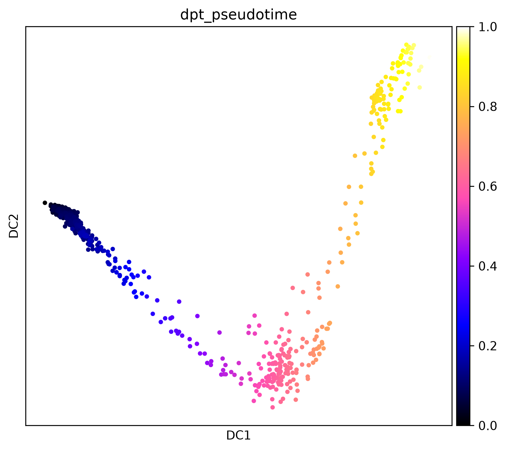
Diffusion pseudotime, 0 at the root cell in the Adipo-CAR cloud and 1 at the far end of the osteolineage arm.

8.3 The sub-populations

The sub-states we are considering were identified using canonical markers: adipogenic CAR cells (Lepr, Cxcl12, Apoe, Lpl, Cebpa, Pparg), a transitional state (Spp1, Ncam1, Kcnk2) and osteolineage cells (Bglap, Sp7, Dcn, Thbs1, Tnn).

markers = {
    "Adipo_CAR":    ["Lepr", "Cxcl12", "Apoe", "Lpl", "Cebpa", "Pparg"],
    "transitional": ["Spp1", "Ncam1", "Kcnk2"],
    "OLC":          ["Bglap", "Sp7", "Dcn", "Thbs1", "Tnn"],
}
sc.pl.dotplot(
    msc,
    groupby="sub_annotation",
    var_names=[g for v in markers.values() for g in v],
    standard_scale="var",
)

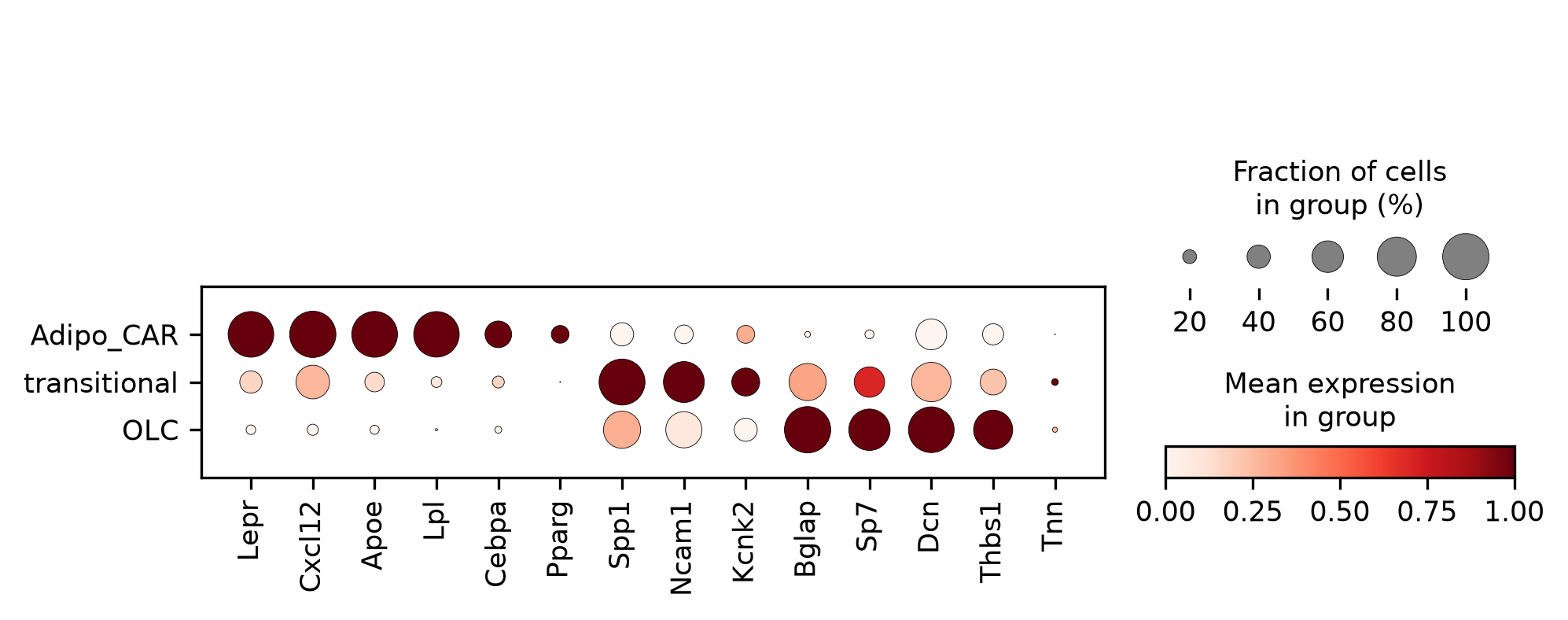
Marker expression per sub-population, scaled per gene. Spp1, Ncam1 and Kcnk2 peak in the transitional state, which also carries intermediate levels of both the adipogenic and the osteolineage programme.

Split by condition

The ridge models and the knockout simulations are run separately per condition, so we write one object per condition next to the full subset.

msc.write(PERT / "MSCs_diffmap_subset.h5ad")
msc[msc.obs["Condition"] == "WT"].copy().write(PERT / "MSCs_diffmap_WT_subset.h5ad")
msc[msc.obs["Condition"] == "KO"].copy().write(PERT / "MSCs_diffmap_KO_subset.h5ad")

To keep this example simple, we run the following steps only on the KO subset (312 cells: 222 Adipo-CAR, 64 transitional, 26 OLC).

Next: Ridge models and KO simulations