Installation
# Install from CRAN:
install.packages("CimpleG")

# Install dev version from github:
devtools::install_github("costalab/CimpleG")
Getting started
library("CimpleG")

data(train_data)
data(train_targets)
data(test_data)
data(test_targets)

# check the train_targets table to see
# what other columns can be used as targets
# colnames(train_targets)

# mini example with just 4 target signatures
set.seed(42)
cimpleg_result <- CimpleG(
  train_data = train_data,
  train_targets = train_targets,
  test_data = test_data,
  test_targets = test_targets,
  method = "CimpleG",
  has_annotation = TRUE,
  target_columns = c(
    "neurons",
    "glia",
    "blood_cells",
    "fibroblasts"
  )
)

cimpleg_result$results
# check generated signatures
cimpleg_result$signatures
#>      neurons         glia  blood_cells  fibroblasts
#> "cg24548498" "cg14501977" "cg04785083" "cg03369247"
Get signature annotation
# Get it directly from the results object
cimpleg_result$annotation
#> # A tibble: 4 × 8
#>   IlmnID     CHR_hg38 Start_hg38  End_hg38 UCSC_RefGene_Name  UCSC_RefGene_Group
#>   <chr>      <chr>         <dbl>     <dbl> <chr>              <chr>
#> 1 cg24548498 chr2      181684680 181684682 <NA>               <NA>
#> 2 cg14501977 chr12     123948446 123948448 CCDC92             5'UTR
#> 3 cg04785083 chr1        8971202   8971204 CA6                Body
#> 4 cg03369247 chr8       20174518  20174520 SLC18A1;SLC18A1;S… Body;Body;Body;Bo…
#> # ℹ 2 more variables: UCSC_CpG_Islands_Name <chr>,
#> #   Relation_to_UCSC_CpG_Island <chr>

# or idependently through the "get_cpg_annotation" function
signature_annotation <- get_cpg_annotation(cimpleg_result$signatures)

# check signature annotation
signature_annotation
#> # A tibble: 4 × 8
#>   IlmnID     CHR_hg38 Start_hg38  End_hg38 UCSC_RefGene_Name  UCSC_RefGene_Group
#>   <chr>      <chr>         <dbl>     <dbl> <chr>              <chr>
#> 1 cg24548498 chr2      181684680 181684682 <NA>               <NA>
#> 2 cg14501977 chr12     123948446 123948448 CCDC92             5'UTR
#> 3 cg04785083 chr1        8971202   8971204 CA6                Body
#> 4 cg03369247 chr8       20174518  20174520 SLC18A1;SLC18A1;S… Body;Body;Body;Bo…
#> # ℹ 2 more variables: UCSC_CpG_Islands_Name <chr>,
#> #   Relation_to_UCSC_CpG_Island <chr>
Plot generated signatures
# adjust target names to match signature names

# check generated signatures
plt <- signature_plot(
  cimpleg_result,
  train_data,
  train_targets,
  sample_id_column = "gsm",
  true_label_column = "cell_type"
)
print(plt$plot)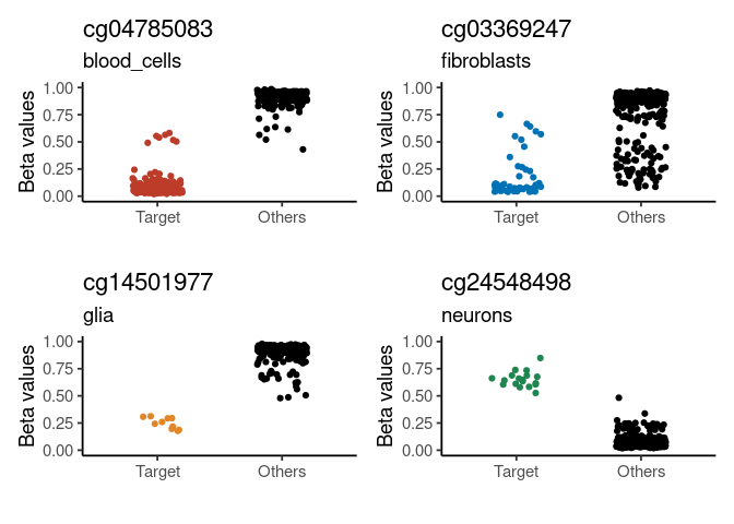
Difference of means vs Sum of variances (dmsv) plots
We have two different functions to produce these plots, one with a simpler interface (and arguably cleaner look) than the other. I might unify these interfaces in the future.
basic plot
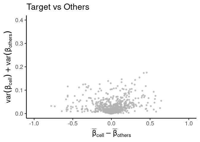
plt <- diffmeans_sumvariance_plot(
  data = train_data,
  target_vector = train_targets$neurons == 1
)
print(plt)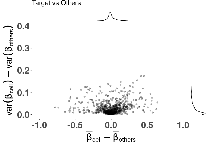
adding color, highlighting selected features
df_dmeansvar <- compute_diffmeans_sumvar(
  data = train_data,
  target_vector = train_targets$neurons == 1
)

parab_param <- .7

df_dmeansvar$is_selected <- select_features(
  x = df_dmeansvar$diff_means,
  y = df_dmeansvar$sum_variance,
  a = parab_param
)
With the simpler interface
plt <- dmsv_plot(
  dat = df_dmeansvar,
  label_var1 = "Neurons",
  highlight_var = "is_selected",
  display_var = "is_selected",
  point_color = "purple"
)
print(plt)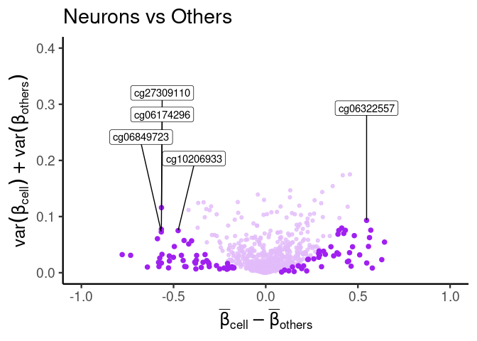
With the more complex interface
plt <- diffmeans_sumvariance_plot(
  data = df_dmeansvar,
  label_var1 = "Neurons",
  color_all_points = "purple",
  threshold_func = function(x, a) (a * x)^2,
  is_feature_selected_col = "is_selected",
  func_factor = parab_param
)
print(plt)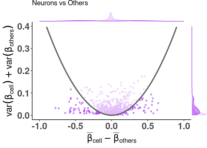
labeling specific features
# labeling best signature found by CimpleG
df_dmeansvar$best_neuron_sig <- (df_dmeansvar$id %in% cimpleg_result$signatures["neurons"])

plt <- dmsv_plot(
  dat = df_dmeansvar,
  label_var1 = "Neurons",
  highlight_var = "is_selected",
  display_var = "best_neuron_sig",
  point_color = "red"
)
print(plt)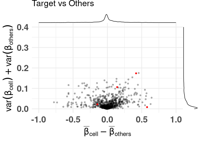
Deconvolution plots
mini example with just 4 signatures
deconv_result <- run_deconvolution(
  cpg_obj = cimpleg_result,
  new_data = test_data
)

plt <- deconvolution_barplot(
  deconvoluted_data = deconv_result,
  meta_data = test_targets,
  sample_id = "gsm",
  true_label = "cell_type"
)
print(plt$plot)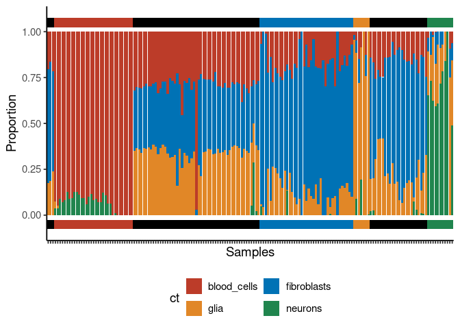
Benchmarking example
This example is a little more advanced
first lets create additional deconvolution results so that we can compare them
In this example, we’ll create two additional models made with CimpleG. One using only hypermethylated signatures, and the other using 3 CpGs per signature instead of just one. Then we will benchmark them against eachother. This is similar to the approach that we use in the paper except there we use real data.
set.seed(42)
cimpleg_hyper <- CimpleG(
  train_data = train_data,
  train_targets = train_targets,
  test_data = test_data,
  test_targets = test_targets,
  method = "CimpleG",
  pred_type = "hyper",
  target_columns = c(
    "neurons",
    "glia",
    "blood_cells",
    "fibroblasts"
  )
)
#> Training for target 'neurons' with 'CimpleG' has finished.: 0.251 sec elapsed
#> Training for target 'glia' with 'CimpleG' has finished.: 0.253 sec elapsed
#> Training for target 'blood_cells' with 'CimpleG' has finished.: 0.29 sec elapsed
#> Training for target 'fibroblasts' with 'CimpleG' has finished.: 0.268 sec elapsed

deconv_hyper <- run_deconvolution(
  cpg_obj = cimpleg_hyper,
  new_data = test_data
)


set.seed(42)
cimpleg_3sigs <- CimpleG(
  train_data = train_data,
  train_targets = train_targets,
  test_data = test_data,
  test_targets = test_targets,
  method = "CimpleG",
  n_sigs = 3,
  target_columns = c(
    "neurons",
    "glia",
    "blood_cells",
    "fibroblasts"
  )
)
#> Training for target 'neurons' with 'CimpleG' has finished.: 0.315 sec elapsed
#> Training for target 'glia' with 'CimpleG' has finished.: 0.296 sec elapsed
#> Training for target 'blood_cells' with 'CimpleG' has finished.: 0.349 sec elapsed
#> Training for target 'fibroblasts' with 'CimpleG' has finished.: 0.307 sec elapsed

deconv_3sigs <- run_deconvolution(
  cpg_obj = cimpleg_3sigs,
  new_data = test_data
)remember this is just an example, the results themselves are meaningless!
deconv_3sigs$prop_3sigs <- deconv_3sigs$proportion
deconv_hyper$prop_hyper <- deconv_hyper$proportion
deconv_result$prop_cimpleg <- deconv_result$proportion

dummy_deconvolution_data <-
  deconv_result |>
  dplyr::mutate(true_vals = proportion + runif(nrow(deconv_result), min = -0.1, max = 0.1)) |>
  dplyr::select(cell_type, sample_id, prop_cimpleg, true_vals) |>
  dplyr::left_join(deconv_hyper |> dplyr::select(-proportion), by = c("sample_id", "cell_type")) |>
  dplyr::left_join(deconv_3sigs |> dplyr::select(-proportion), by = c("sample_id", "cell_type")) |>
  dplyr::mutate_if(is.numeric, function(x) {
    ifelse(x < 0, 0, x)
  }) |>
  dplyr::mutate_if(is.numeric, function(x) {
    ifelse(x > 1, 1, x)
  }) |>
tibble::as_tibble()first we can check how the true values compare against the predicted values
scatter_plts <- CimpleG:::deconv_pred_obs_plot(
  deconv_df = dummy_deconvolution_data,
  true_values_col = "true_vals",
  predicted_cols = c("prop_cimpleg", "prop_hyper", "prop_3sigs"),
  sample_id_col = "sample_id",
  group_col = "cell_type"
)
scatter_panel <- scatter_plts |> patchwork::wrap_plots(ncol = 1)

print(scatter_panel)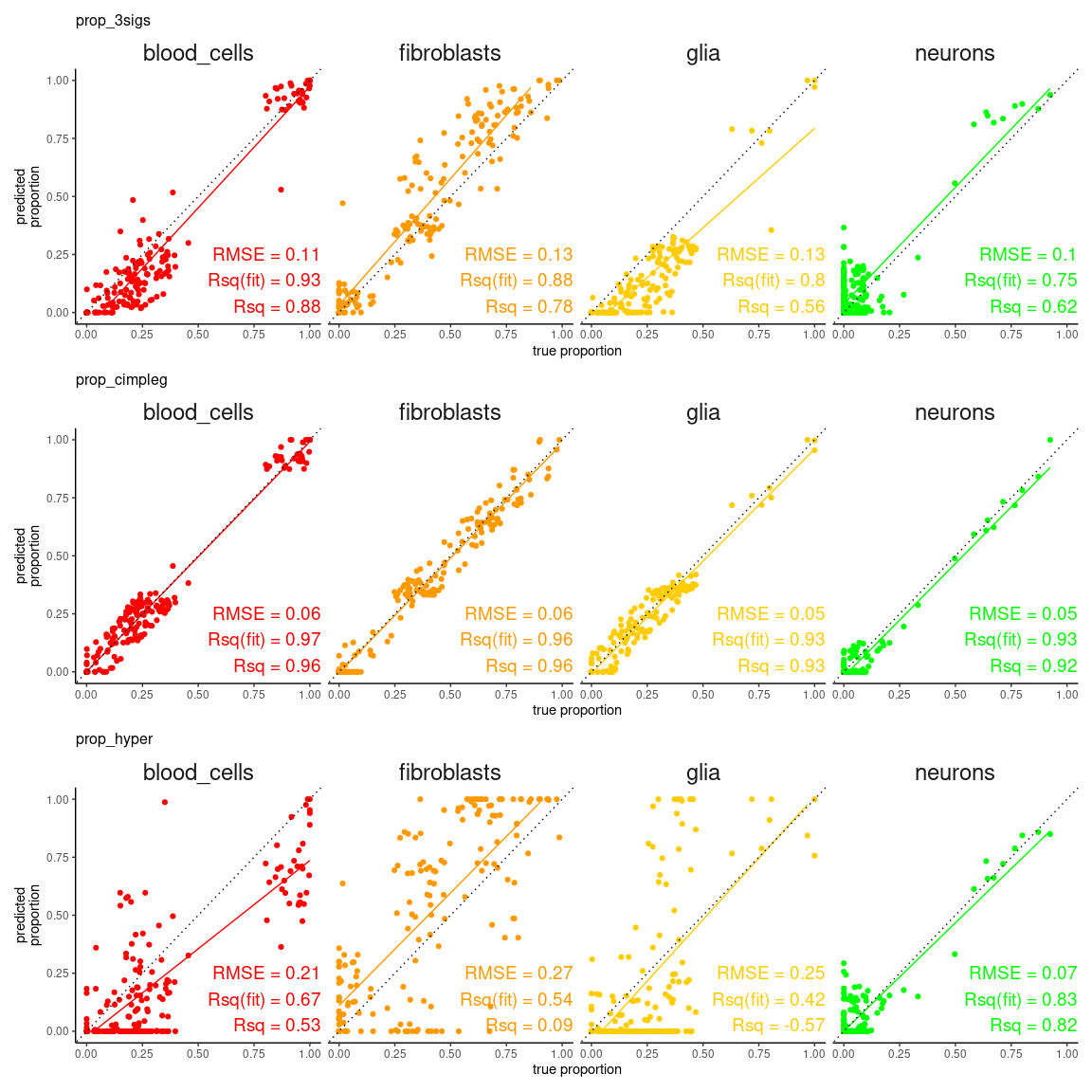
now, more interestingly, we can see in detail and rank one of the measures used to evaluate the deconvolution results
rank_plts <- CimpleG:::deconv_ranking_plot(
  deconv_df = dummy_deconvolution_data,
  true_values_col = "true_vals",
  predicted_cols = c("prop_cimpleg", "prop_hyper", "prop_3sigs"),
  sample_id_col = "sample_id",
  group_col = "cell_type",
  metrics = "rmse"
)
rank_panel <- list(rank_plts$perf_boxplt[[1]], rank_plts$nemenyi_plt[[1]]) |> patchwork::wrap_plots()

print(rank_panel)![]()